Understanding JavaScript Object Notation (JSON)

 One of the most useful things you might want to learn when understanding how to present your data with D3 is how to *structure* your data so that it is easy to use.

As explained in an earlier post, there are several different types of data that can be requested by D3 including text, Extensible Markup Language, (xml), HyperText Markup Language (html), Comma Separated Values (csv), Tab Separated Values (tsv) and JavaScript Object Notation (json).

Comma separated variables and tab separated variables are a fairly well understood form of data. It is expressed as rows and columns of information that is separated using a known character. While this form of data is simple to understand, it is not easy to incorporate a hierarchy structure to the data, and when you try, it isn't natural and makes managing the data difficult.

JavaScript Object Notation (JSON) presents a different mechanism for storing data. A light weight description could read "JSON is a text-based open standard designed to present human-readable data. It is derived from the JavaScript scripting language, but it is language and platform independent."

Unfortunately, when I first started using JSON, I struggled with the concept of how it was structured, in spite of some fine descriptions on the web (start with http://www.json.org/ in my humble opinion). So the following is how I came to think of and understand JSON.

Fair Warning: This advice is no substitute for the correct explanation of the topic of data structures that I'm sure you could receive from a reputable educational site or institution. It's just the way I like to think of it :-). It's also just the way that I *started* to understand JSON. There is plenty to learn and understand once you grasp the basics. So this isn't a complete guide. Just the beginnings.

In the following steps we'll go through a process that (hopefully) demonstrates that we can transform identifiers that would represent the closing price for a stock of 58.3 on 2013-03-14 into more traditional x,y coordinates.

I think of data as having an identifier and a value.

 identifier: value

 If a point on a graph is located at the x,y coordinates 150,25 then the identifier 'x' has a value 150.

 "x": 150

 If the x axis was a time-line, the true value for 'x' could be "2013-03-14".

 "x": "2013-03-14"

 This example might look similar to those seen by users of d3.js, since if we're using date / time format we can let D3 sort out the messy parts like what coordinates to provide for the screen.

And there's no reason why we couldn't give the 'x' identifier a more human readable label such as "date". So our data would look like;

 "date": "2013-03-14"

 This is only one part of our original x,y = 150,25 data set. The same way that the x value represented a position on the x axis that was really a date, the y value represents a position on the y axis that is really another number. It only gets converted to 25 when we need to plot a position on a graph at 150,25. If the 'y' component represents the closing price of a stock we could take the same principles used to transform...

 "x": 150

 ... into ...

 "date": "2013-03-14"

 ... to change ....

 "y": 25

 ... into ...

 "close": 58.3

 This might sound slightly confusing, so try to think of it this way. We want to plot a point on a graph at 150,25, but the data that this position is derived from is really "2013-03-14", 58.3. D3 can look after all the scaling and determination of the range so that the point gets plotted at 150,25 and our originating data can now be represented as;

 "date": "2013-03-14", "close": 58.3

 This represents two separate pieces of data. Each of which has an identifier ("date" or "close") and a value ("2013-03-14" and 58.3)

If we wanted to have a series of these data points that represented several days of closing prices, we would store them as an array of identifiers and values similar to this;

{ "date": "2013-03-14", close: 58.13 },
{ "date": "2013-03-15", close: 53.98 },
{ "date": "2013-03-16", close: 67.00 },
{ "date": "2013-03-17", close: 89.70 },
{ "date": "2013-03-18", close: 99.00 }

 Each of the individual elements of the array is enclosed in curly brackets and separated by commas.

I am making the assumption that you are familiar with the concept of what an 'array' is. If this is an unfamiliar word, in the context of data, then I strongly recommend that you do some Goggling to build up some familiarity with the principle.

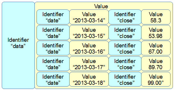
Now that we have an array, we can apply the same rules to it as we did the the item that had a single value. We can give it an identifier all of its own. In this case we will call it "data". Now we can use our identifier: value analogy to use "data" as the identifier and the array as the value.

 { "data": [
  { "date": "2013-03-14", close: 58.13 },
  { "date": "2013-03-15", close: 53.98 },
  { "date": "2013-03-16", close: 67.00 },
  { "date": "2013-03-17", close: 89.70 },
  { "date": "2013-03-18", close: 99.00 }
] }

 The array has been enclosed in square brackets to designate it an an array and the entire identifier: value sequence has been encapsulated with curly braces (much the same way that the subset "date", "close" values were enclosed with curly braces.

If we try to convey the same principle in a more graphical format, we could show our initial identifier and value for the x component like so;

 The we can add our additional component for the y value;

 We can then add several of these combinations together in an array;

 Then the array becomes a value for another identifier "data";

 More complex JSON files will have multiple levels of identifiers and values arranged in complex hierarchies which can be difficult to interpret. However, laying out the data in a logical way in a text file is an excellent way to start to make sense of the data.